In the program development, we often encounter a tree structure to represent the relationship between certain data, such as the organizational structure of the enterprise, the classification of goods, operation columns, etc., the current relational database is to store data in the form of two-dimensional table records, and the tree structure of the data must be stored in the two-dimensional table Schema design. Recently, we have been interested in this area, and we are dedicated to sorting out the following common tree structure data.

Adjacency List Pattern Adjacency List
The simplest method is: Adjacency List (Adjacency List pattern). It simply describes the parent node of a node based on the inheritance relationship between nodes, thus creating a two-bit relationship table. The table structure is usually designed as {Node_id,Parent_id}, as follows.

Approximate code for using the join table.
|
|
Using this function for the root node of the entire structure (Food) will print out the entire multilevel tree structure. Since Food is the root node its parent is empty, so call it like this: display_children(",0). will display the entire tree. If you want to display only a part of the whole structure, say the fruit part, call it like this: display_children(‘Fruit’,0);
Using almost the same method we can know the path from the root node to any node. For example, Cherry’s path is “Food >; Fruit >; Red”. To get such a path we need to start from the deepest level “Cherry”, query its parent node “Red” and add it to the path, then we query Red’s parent node and add it to the path as well. And so on up to the highest level “Food”
Here is the code.
|
|
If you use this function for “Cherry”: print_r(get_path(‘Cherry’)), you will get an array like this
The advantages of this scheme are obvious: the structure is simple and easy to understand, and since the relationship between them is maintained by a single parent_id, it is very easy to add, delete, and change only the records directly related to it. The disadvantage of course is also very prominent: since the inheritance relationship between nodes is directly recorded, any CRUD operation on the Tree will be inefficient, mainly due to the frequent “recursive” operations, where the recursive process constantly accesses the database and each database IO has a time overhead. For example, if you want to return all the fruits, that is, all the children nodes of the fruits, a seemingly simple operation, you need to use a bunch of recursion. Of course, this scheme is not useless, when the tree level is relatively small is very practical, based on the neighbor list pattern can also be expanded is a flat table, the difference is the level of the node and the order of the current node is also put into the table, more suitable for similar comments and other scenarios, the specific table structure similar to this, here will not elaborate in depth.

Path Enumeration
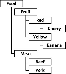
The materialized path is actually easier to understand, it is actually the full path of the node that is recorded when the node is created. The following figure is an example.

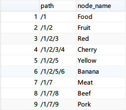
The result of storing according to Path Enumeration is as follows.

This solution is based on the idea of unix file directories, and mainly trades space for time.
Query all the children nodes under a certain node: (Take Fruit as an example)
How to query direct child nodes? MySQL regular expression query is needed for.
Query all superiors of any node: (take Yellow as an example).
Insert additional data.
The disadvantage of this scheme is that the depth of the tree may exceed the length of the PATH field, so the maximum depth it can support is not infinite.
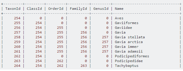
If the number of hierarchies is determined, all columns can be expanded again, as shown below, which is more tried for content with determined hierarchies like administrative divisions, biological taxonomy (boundary, phylum, order, family, genus, species).

Closure Table
Closure Table is a more thorough full path structure that records the full expansion form of related nodes on the path respectively. It can clarify the relationship between any two nodes without redundant queries, and cascade deletion and node movement are also very convenient. But its storage overhead will be larger, in addition to the Meta information of the nodes, but also need a special relationship table.
The following diagram gives an example of data example.

Create master table.
Create relationship tables.
where
- Ancestor represents an ancestor node
- Descendant represents the descendant node
- Distance Ancestor is the distance from Descendant
Adding data (creating a stored procedure)
|
|
The data in the 2 tables after completion looks roughly like this: (Note: each node has a record to itself.)


Query all child nodes under Fruit.
Query the direct child nodes under Fruit.
Query the tier that Fruit is in.
It is also very simple to delete nodes, so I will not elaborate much here.
Left and Right Value Coding Nested Set
In general database based applications, the need for queries is always greater than that for deletions and modifications. In order to avoid the “recursive” process of querying a tree structure, we design a new non-recursive querying, infinitely grouped left and right value encoding scheme based on Tree’s preorder traversal to save the data of the tree.

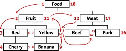
The first time you see this table structure, I believe most people are not sure how the left value (Lft) and right value (Rgt) are calculated, and this table design does not seem to preserve the inheritance relationship between parent and child nodes. But when you point your finger at the numbers in the table and count from 1 to 18, you should find something, right? Yes, the order in which you move your finger is the order in which the tree is traversed in preorder, as shown in the figure below. When we start from the left side of the root node Food, marked as 1, and along the direction of the traversal of the previous order, in order to mark the numbers on the traversal path, we finally came back to the root node Food, and wrote 18 on the right side.

Based on this design, we can infer that all nodes with left values greater than 2 and right values less than 11 are the successor nodes of Fruit, and the structure of the whole tree is stored by the left and right values. However, this is not enough, our aim is to be able to perform CRUD operations on the tree, i.e., we need to construct the relevant algorithm to go with it. The tree is traversed in depth-first, left-to-right order, and each node is labeled with a left value and a right value starting from 1, and these two values are stored in the corresponding name.
How to query?
- Get all the children nodes under a node, take Fruit as an example.
|
|
- Get the total number of descendant nodes
Total number of children = (right value - left value - 1)/2, take Fruit as an example, its total number of children is: (11-2-1)/2 = 4
- Get the number of levels the node is at in the tree, taking Fruit as an example.
|
|
- Get the path where the current node is located, taking Fruit as an example.
|
|
In our daily processing we often also encounter the need to obtain the immediate superior, sibling, or immediate subordinate of a node. To better describe the hierarchical relationship, we can create a view for Tree, adding a hierarchical column whose value can be calculated by writing a custom function.
|
|
After adding the function, we create an a-view and add the new hierarchical column.
- Get the parent node of the current node, using Fruit as an example.
|
|
- Get all direct child nodes, taking Fruit as an example.
|
|
- Get all sibling nodes, using Fruit as an example.
|
|
- Return all leaf nodes
|
|
How to create a tree? How to add data?
The above has described how to retrieve the results, so how can we add new nodes?
The most important thing about Nested set is that there must be a root node as the starting point of all nodes, and usually this node is not used. In order to control the query level, it is recommended to add the parent_id when building the table together with the linked list method.
|
|
|
|
Add a child node (at the start of the child node). Take the example of adding a child node Fruit under Food.
|
|
If you need to append at the end, you need to do the following (for example, add Apple under Red).
|
|
Add a sibling node after node A (for example, add Green after Yellow)
|
|
The above discussion of adding nodes refers to adding end nodes, i.e., the node inserted is not the parent node of the currently existing node. What should we do if we need to insert a non-end node?
The process can be divided into 2 steps: first add a new node, and then move the required node to the lower level of the new node. Node movement method (for example, moving Apple to Yellow).
|
|
delete nodes (including child nodes)
|
|
What if I need to delete only that node and the child nodes are automatically moved up one level?
|
|
The above is the CURD operation of Nested Set, specifically in the use of the recommended combination of transactions and stored procedures together. The advantage of this solution is that it is very convenient to query, but the disadvantage is that each insertion and deletion of data involves too many updates, and if the tree is very large, it may take a long time to insert a piece of data.
interval nested Nested Intervals
The previous introduced the left and right value encoding, I wonder if you have noticed that if the data is huge, each update needs to update almost the entire table, less efficient no better way? Today we will study the interval nesting method.
interval nesting method principle
If the node interval [clft, crgt] and [plft, prgt] have the following relationship: plft <= clft and crgt >= prgt, then the points in the interval [clft, crgt] are the children of [plft, prgt]. Based on this assumption, we can obtain new intervals by continuously scribing down the interval. For example, if there is a blank interval [lft1, rgt1] in the interval [plft, prgt], to add an interval of the same level as [plft,lft1], [rgt1,prgt], just insert the nodes: [(2lft1+rgt1)/3, (rgt1+2lft)/3]. After adding the nodes we are left with [lft1,(2lft1+rgt1)/3] and [(rgt1+2lft)/3,rgt1] two free spaces to add more child nodes.

If we put the intervals in the two-bit plane and treat rgt as the x-axis and lft as the y-axis, then the number of nested intervals is almost like this

Each node [lft, rgt] has children that are contained in y >= lft & x <= rgt. Also the space where y >= clft & x <= crgt is located is a subset of y >= plft & x <= prgt. In addition, since the new right intervals are smaller than the existing left intervals, the new nodes are below the line y = x.
Interval nesting method implementation
After understanding the principle of the interval nesting method, we will consider how to implement it, in principle, the initial interval can use any interval, here we use [0,1] as the root interval.

First, we define 2 points in the XY plane. Depth-first set point and breadth-finite set point for the point <x=1,y=1/2> with depth-first set point <x=1,y=1> and breadth-first set point <x=1/2,y=1/2>. Next, we define the position of the first child node as the midpoint between the parent node and the depth-first set point. The sibling node is the midpoint from the previous child node to the breadth-first set point, as shown in the figure above, where node 1.2 is at <x=3/4, y=5/8>.
Also looking closely we can see the relationship between the points. Also if we know the sum of x and y, we can invert the value of x,y (what is the exact logic, I haven’t figured it out yet either, any of you who know can help explain).
Let’s take the node <x=3/4, y=5/8> as an example, we can get his sum to 11/8.
We define 11 as the numerator (numerator) and 8 as the denominator (denominator), then the numerator of point x is
|
|
The denominator of point x is.
|
|
Molecules at point Y.
|
|
Denominator of Y.
|
|
Next, let’s test whether X and Y can be decoded.

The result is identical to the position of node 1.2 as <x=3/4, y=5/8>. Now we know that only one fraction is needed to represent a point on the plane.
If there is already a fraction 11/8 how do we get the parent of that node? (If the numerator is 3, it means it is the root node)
|
|
|
|
Calculate the position of the current node at the sibling level.
|
|
With the method of querying the parent node and the position of the current node in the same level, the path of the node can be calculated by the combination of these two methods.
After adding the above method and testing, it returns [Err] 1424 - Recursive stored functions and triggers are not allowed. That is, MySQL’s custom functions do not support recursive queries.
|
|
The result of SELECT path (11, 8) is 1.2
Calculate the node hierarchy by
|
|
We know how to convert the encoded nodes into directory form, how to reverse it? The following is the method.
First add 2 helper functions.
To write the reversal function again.
|
|
|
|
select CONCAT(path_numer(‘2.1.3′),’/’,path_denom(‘2.1.3’)) The result is 51/64
Reference link.
- http://salman-w.blogspot.com/2012/08/php-adjacency-list-hierarchy-tree-traversal.html
- https://packagist.org/search/?tags=adjacency%20list
- https://communities.bmc.com/docs/DOC-9902
- https://coderwall.com/p/lixing/closure-tables-for-browsing-trees-in-sql
- https://www.sitepoint.com/hierarchical-data-database/
- https://packagist.org/search/?q=Nested+Set
- http://www.rampant-books.com/art_vadim_nested_sets_sql_trees.htm